Electromagnetic engineering software

DAD FieldWorks

Your geometry, calculation and results.
Connected in one workspace.

Work with antenna structures, waveguides and PCB models through an integrated desktop workflow. Move from editable geometry to electric and magnetic fields, currents and RF responses.

Parametric modelling

Start with
the geometry.

Edit dimensions, expressions and placements directly on model objects. Keep geometry, material assignments and source definitions together.

Prepare ports and mesh controls for the calculation. Include ideal capacitive and inductive loads in supported Direct MoM models.

Native calculation methods

A method for
the model.

Choose the calculation route for your geometry, excitation and quantities of interest.

FEMFinite Element Method
Harmonic volume field analysis with modal excitation and electric and magnetic field inspection.
FDTDFinite Difference Time Domain
Time domain calculation and exploration of stored electric and magnetic field components.
MoMMethod of Moments
Direct electromagnetic analysis of conducting surfaces, with current and network results.
MLFMMMultilevel Fast Multipole Method
Multilevel interaction evaluation for MoM surface calculations, combining direct near interactions with a hierarchy for distant interactions.

Inside the application

See what the model reveals.

Explore field distributions and antenna radiation. Inspect complex responses in Cartesian, polar and Smith views, place markers and export numerical data.

Electric fields in the model.
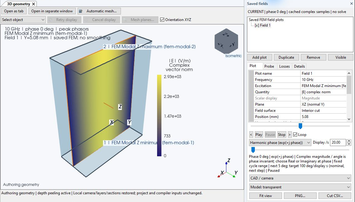
WR90 electric field at 10 GHz for modal excitation 1, with the XZ slice and V/m legend.
WR90 waveguide at 10 GHz. Electric field on an XZ slice at Y = 5.08 mm, in V/m.

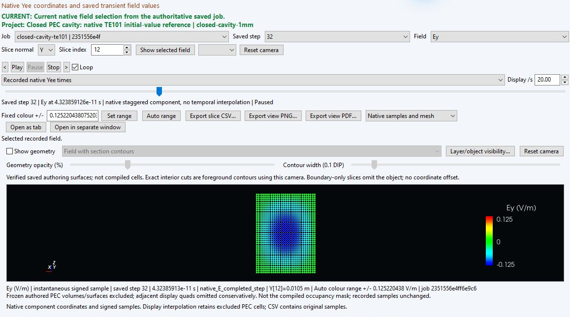
Follow the time domain.

Native FDTD Ey samples and mesh of a closed PEC cavity at time step 32 and Y = 10.5 mm, in V/m.
Closed PEC cavity. Native Ey samples at time step 32, approximately 43.24 ps, in V/m.

See currents on conducting surfaces.
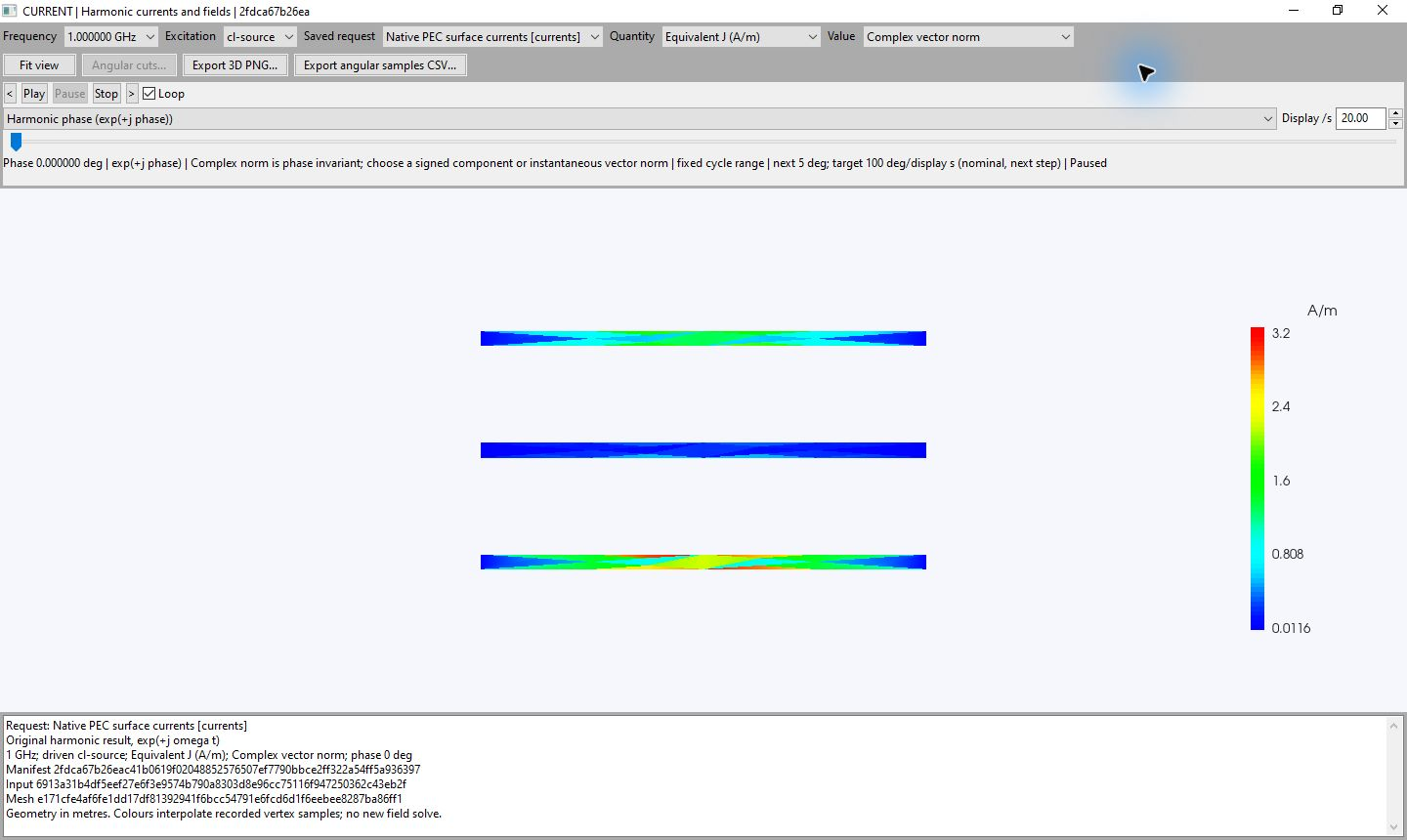
DAD FieldWorks showing native Direct MoM surface current on three PEC strips at 1 GHz, with an A/m legend.
Three coupled PEC strips at 1 GHz. Equivalent J is shown as a complex vector norm in A/m.

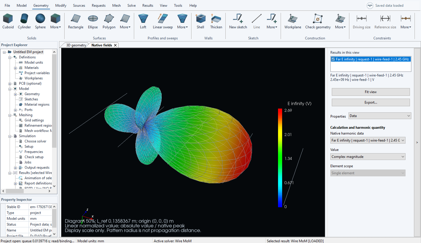
Explore the radiation pattern.

DAD FieldWorks showing the Yagi antenna far field at 2.45 GHz, with the complex magnitude of E infinity in V, its colour scale and the result controls on the right.
Yagi antenna far field at 2.45 GHz. A saved Wire MoM result in DAD FieldWorks.

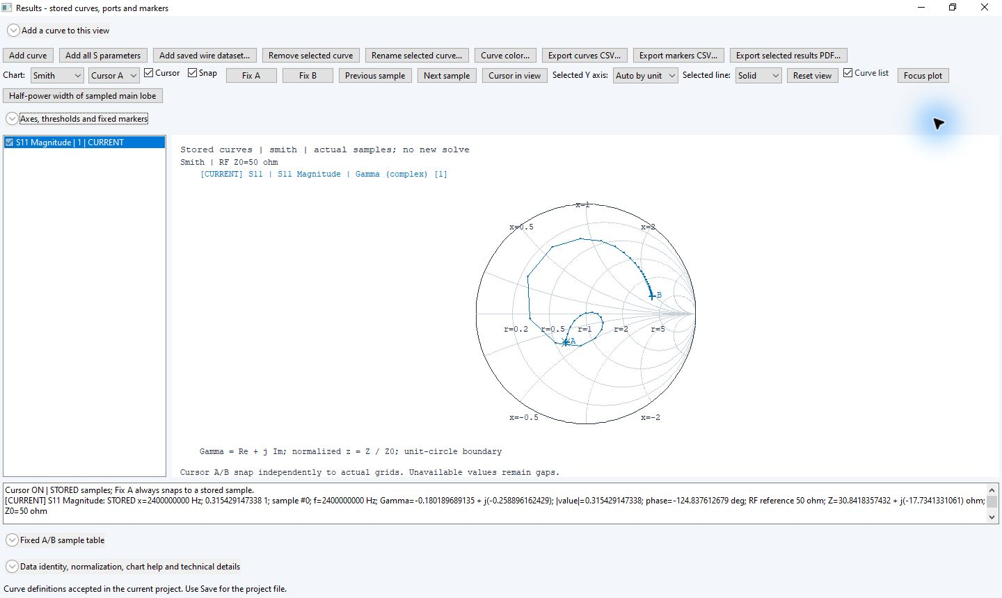
Read the complex RF response.

Smith chart of the five element Yagi reflection response from 2.40 to 2.80 GHz, with a 50 ohm RF reference.
Yagi reflection response from 2.40 to 2.80 GHz, referenced to 50 ohms.

Original application views of saved DAD FieldWorks calculations. Results for selected benchmark cases have been verified through comparison with established electromagnetic simulation software.

Aircraft scattering · 30 MHz

Scattered fields.
Surface currents.

Explore saved results for a simplified civil aircraft illuminated by a plane wave. View the scattered far field together with the physical surface current density on the conducting model.
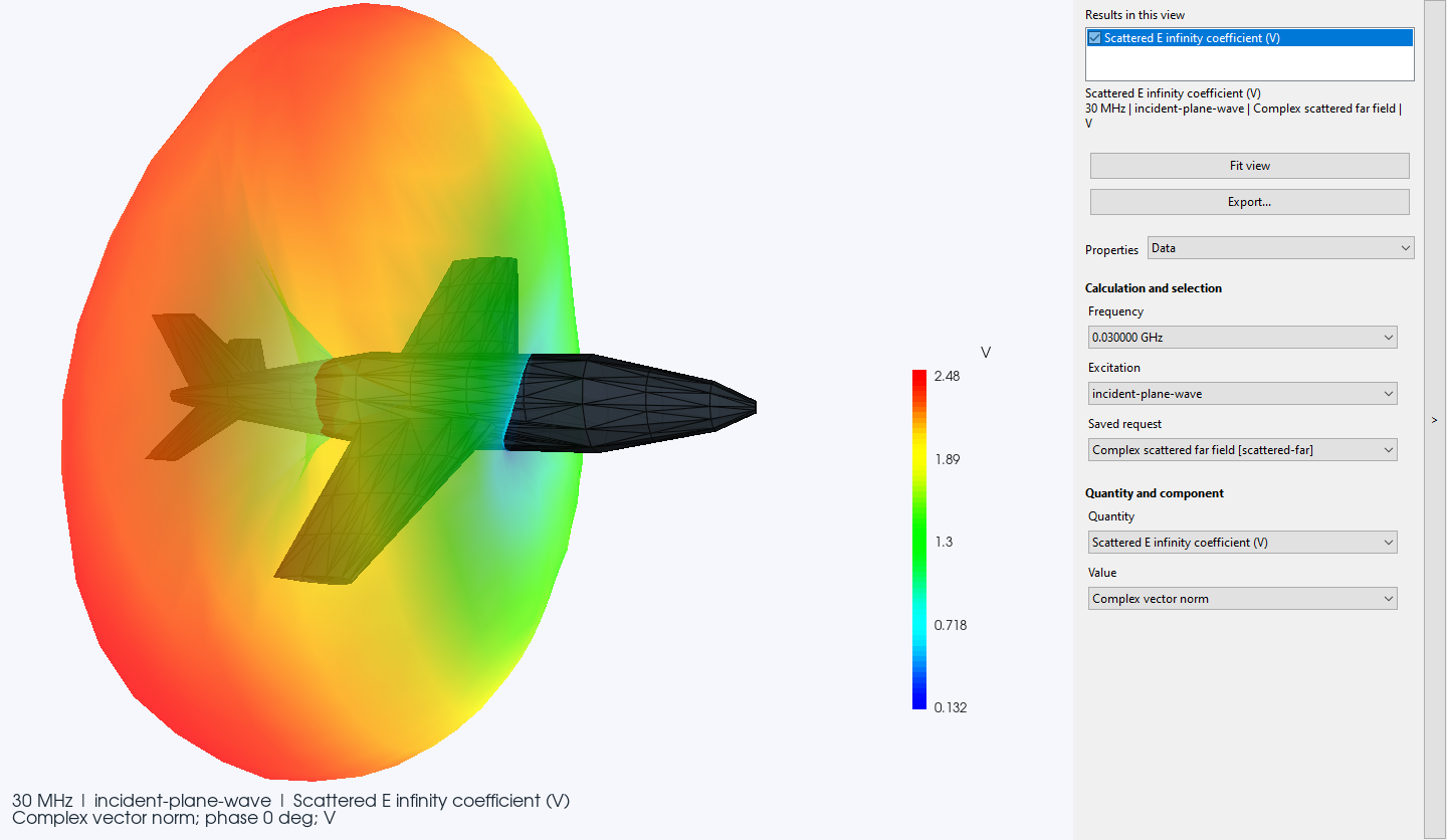
DAD FieldWorks showing a simplified aircraft and its scattered electric far field at 30 MHz under plane wave illumination, with a colour scale from 0.132 to 2.48 V.
Plane wave scattering from a simplified civil aircraft at 30 MHz. Complex vector norm of the scattered electric far field coefficient, in V.

Inspect the current on the surface.

The current view shows the physical PEC surface current density in A/m. Its colour legend is separate from the far field coefficient in V.
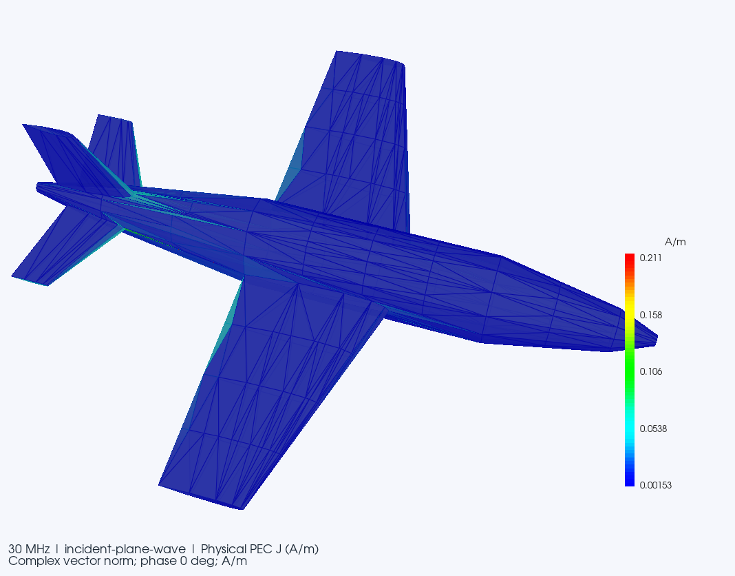
Physical surface current30 MHz · A/m
Physical PEC surface current density on the meshed aircraft at 30 MHz, shown as a complex vector norm with a colour scale from 0.00153 to 0.211 A/m.
Physical PEC surface current density on the simplified aircraft at 30 MHz under plane wave illumination. Complex vector norm, in A/m.

20 metre band · Wire MoM

From the radiation pattern
to the RF response.

Inspect stored far field and reflection results from a dipole project covering 14.0 to 14.5 MHz. Move between the spatial pattern, the mesh overlay and the complex response in the Smith view.
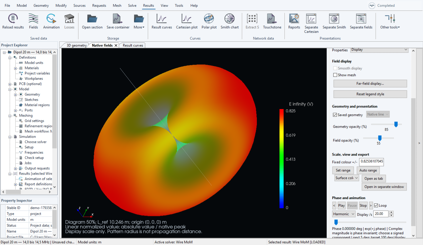
DAD FieldWorks showing the stored far field of a dipole for the 20 metre band without a mesh overlay, with an E infinity legend in V.
Wire MoM far field of a dipole for the 20 metre band, shown without the mesh overlay. The colour scale gives the radiating E coefficient in V.

The field views show the radiating E coefficient in V. Plot radius is normalised for display and does not represent a propagation distance.

Inspect the result in detail.
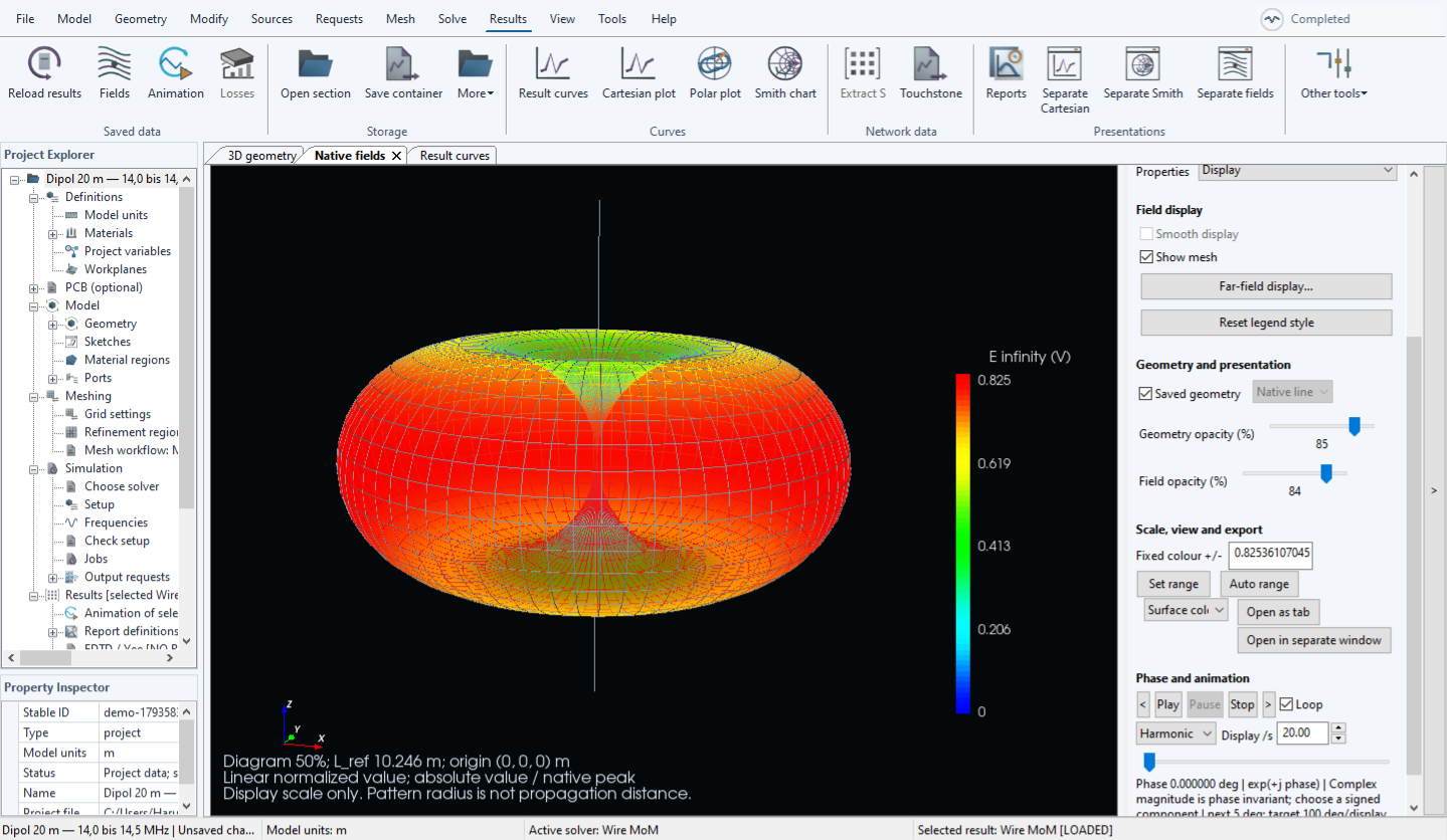
Far field with mesh overlay
Dipole far field in DAD FieldWorks with the mesh overlay visible, the E infinity colour scale and display controls on the right.
The dipole far field with the mesh overlay enabled. The colour scale gives the radiating E coefficient in V.
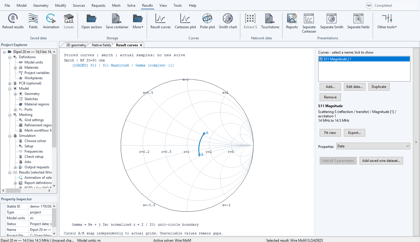
Smith chart14.0 to 14.5 MHz · 50 ohms
Smith chart of the dipole S11 response from 14.0 to 14.5 MHz with a 50 ohm reference and A and B markers.
Dipole S11 response from 14.0 to 14.5 MHz in the Smith view, referenced to 50 ohms. The curve shows the complex reflection coefficient.

Magnetic loop antenna · 14.14 MHz

The complete pattern.
Then every component.

Begin with the complex vector norm of the radiated field. Inspect the signed X, Y and Z components in the detailed views below.
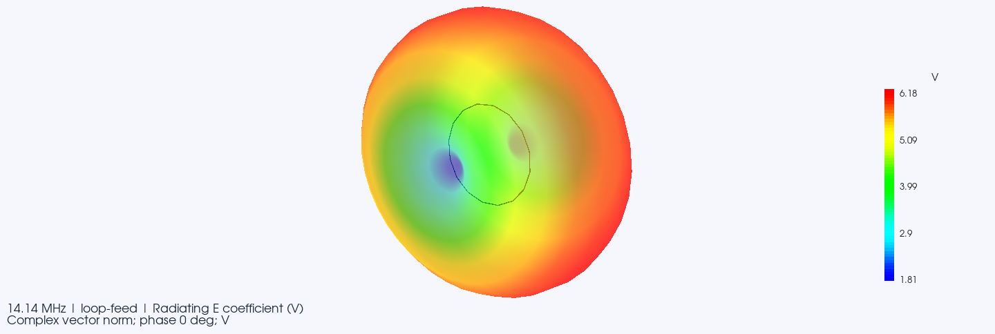
Loop antenna radiation pattern at 14.14 MHz, shown as the complex vector norm with a colour scale from 1.81 to 6.18 V.
Loop antenna at 14.14 MHz. Complex vector norm of the radiating E coefficient, in V. The norm is independent of harmonic phase.

The images show the saved radiating electric field coefficient in V. Plot radius is normalised for display and does not represent a propagation distance.

Full vector decomposition.

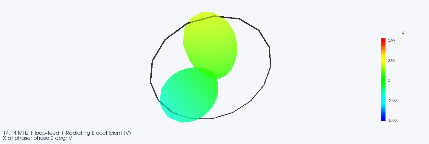
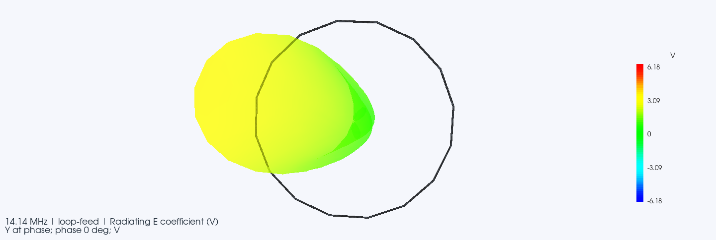
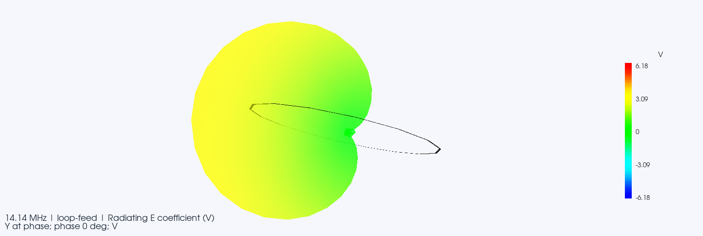
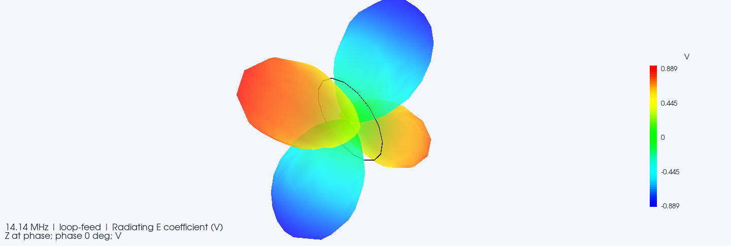
Examine each Cartesian component at harmonic phase 0°, using the convention exp(+jφ). Each view retains its own colour scale for numerical inspection.

X componentPhase 0°
Signed X component of the loop antenna radiating E coefficient at 14.14 MHz and phase 0 degrees, with its colour legend.
14.14 MHz. Signed X component at harmonic phase 0°, in V. Colour scale: −5.99 to +5.99 V.
Y componentPhase 0° · two views
Front view of the signed Y component of the radiating E coefficient at 14.14 MHz and phase 0 degrees.
14.14 MHz. Signed Y component at harmonic phase 0°, front view, in V. Colour scale: −6.18 to +6.18 V.
Oblique view of the same signed Y component at 14.14 MHz and phase 0 degrees, with its colour legend.
14.14 MHz. The same Y component at harmonic phase 0° from another viewing angle. Colour scale: −6.18 to +6.18 V.
Z componentPhase 0°
Four lobes of the signed Z component at 14.14 MHz and phase 0 degrees, with its colour legend. The upper lobe meets the edge of the captured view.
14.14 MHz. Signed Z component at harmonic phase 0°, in V. Colour scale: −0.889 to +0.889 V.
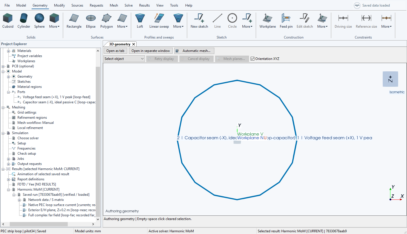
Loop modelling workspaceGeometry and excitation
DAD FieldWorks modelling workspace showing a PEC strip loop, a 1 V peak voltage feed seam and an ideal capacitor seam.
Loop modelling workspace. A PEC strip loop with a voltage feed seam and an ideal capacitive seam.

DAD FieldWorks in motion

Watch the radiation pattern change.

Explore how a Yagi antenna radiates across 2.4 to 2.8 GHz. This recording shows playback of saved simulation results in the application.

Yagi antenna, 2.4 to 2.8 GHz. Saved far field results in DAD FieldWorks. The normalised plot radius represents the radiation quantity, not a physical distance. Open video.

Licensing & pricing

DAD FieldWorks is available on request. Contact DigitalArtDeco Labs for licensing information and a quotation.

Request a quote

DAD FieldWorks application view